Navigator

Model overview 

The MESSAGE-ix-buildings model simulates the energy consumption, material usage, and CO2 emissions of residential and commercial buildings in various global regions. This model combines bottom-up modelling of energy demand, stock turnover dynamics, and discrete choice modelling for energy efficiency decisions, enabling analyzing effects of policy, technological, and behavioral changes. It is coherently connected to the MESSAGEix integrated assessment model and considers variations in geography, socio-economics, and building characteristics. It is open-access, with code, data and a simplified version of documentation available on GitHub.

Link to code/data 

The code and data needed to use it are available from the GitHub public repository:

https://github.com/iiasa/message-ix-buildings 

Publications 

Mastrucci, A., van Ruijven, B., Byers, E., Poblete-Cazenave, M. and Pachauri, S., 2021. Global scenarios of residential heating and cooling energy demand and CO2 emissions. Climatic Change, 168, pp.1-26. 

iTEM Open Database is a harmonized transport database that aims to create transparency through three key features:

• Open Data: Assembling a comprehensive collection of publicly-available transportation data in a harmonized manner.
• Open-Code: All code used for cleaning the datasets is publicly accessible from GitHub and documented. All codes are opened for modification and extension.

• Open Dataset: A harmonized transport data set of historical values.

The iTEM Open Database is composed of individual datasets collected from public sources. Each  dataset  is  downloaded,  cleaned,  and  harmonised  to  the common  region and technology  definitions  defined  by  the  iTEM  consortium https://transportenergy.org. For each  dataset,  we describe the name of the dataset, the web link to the original source, the web link to the cleaning script (in python), variables, and explain the data cleaning steps (which explains the data cleaning script in plain English). These steps are carefully documented in a “Rule Book” (https://zenodo.org/record/4287423/files/iTEM_Open_Data_Rule_Book.pdf?download=1) for documentation purpose so the process is transparent and reproducible.

The iTEM region definition (individual countries including 17 world regions https://github.com/transportenergy/metadata/blob/master/model/regions.) and variables (e.g. activity, energy, emission, stock), service (freight and passenger), mode (e.g. air, rail, road, shipping), vehicle type (e.g. cars, SUV, bus, medium-size trucks) , technology (e.g. battery electric vehicles, fuel cell vehicles, internal combustion engine vehicles), and fuels (e.g. compressed natural gas, biofuels, gasoline, diesel) are harmonized to “iTEM scenarios template.” The “iTEM scenario template” (https://github.com/transportenergy/metadata/blob/main/model/iTEM%20MIP3%20template.csv) is the template developed to harmonize the scenario comparison of future projections.

Python and Jupyter notebooks are the main technologies used for cleaning the datasets. We use Git for version control and GitHub as the service for making the code available to the public. In total, twelve datasets have been made available to date. These datasets include: four datasets about passenger data, five datasets about freight data, and two socio-demographic – population and GDP. List datasets available to date in iTEM Open Database. https://github.com/transportenergy/metadata/tree/main/historical/input

LINK TO CODE

All code and documentation will be publicly accessible and open for modification and extension. https://github.com/transportenergy

LINK TO DATASET

https://zenodo.org/record/4287423#.ZCr0YOxBzX0

LICENSE AGREEMENT

Creative Commons Attribution 4.0 International

We develop a method to place charger locations in Europe that meets the demand of goods movements between regions while following EU driving regulations. The spatial resolution of regions is based on the Nomenclature of Territorial Units for Statistics (NUTS)-3 regions. The annual flow of goods transported by HDV is identified using the ETISplus dataset. We develop a travel pattern for the HDV to convert flows into trip chains with the traversed LHT number. The traveled routes between the regions are mapped. Locations of short period stops, i.e., breaks, and long period stops, i.e., rests, are allocated/assigned along traveled routes to construct a trip chain for each moving HDV. Break and rest locations for all moving HDVs are aggregated to suggest energy requirements if assuming these HDVs are BETs. The aggregated energy to charge stopped BETs is used to identify the number and type of chargers within each suggested charging station.
The presented datasets contain spatial information for generating charger stations with specifications according to charging needs. The datasets contain information about: Transport network model and edges, Transported flows, routes and flow center information data, region centers , and Planned transport infrastructure.

LINK TO DATASET
https://zenodo.org/record/7225261#.ZFyeD-xBzX0

LICENSE AGREEMENT
Creative Commons Attribution 4.0 International

Battery electric vehicles (BEVs) are crucial for a sustainable transportation system. As more people adopt BEVs, it becomes increasingly important to accurately assess the demand for charging infrastructure. However, much of the current research on charging infrastructure relies on outdated assumptions, such as the assumption that all BEV owners have access to home chargers and the “Liquid-fuel” mental model. To address this issue, we simulate the travel and charging demand on three charging behavior archetypes. We use a large synthetic population of Sweden, including detailed individual characteristics, such as dwelling types (detached house vs. apartment) and activity plans (for an average weekday). This data repository aims to provide the BEV simulation’s input, assumptions, and output so that other studies can use them to study sizing and location design of charging infrastructure, grid impact, etc.

LINK TO CODE

https://github.com/TheYuanLiao/synthetic-sweden (Software)

LINK TO DATASET

https://zenodo.org/record/7549847#.ZFydCOxBzX0

LICENSE AGREEMENT

Creative Commons Attribution 4.0 International

The data contains a synthetic replica of over 10 million Swedish individuals (i.e., agents), their household characteristics, and activity-travel plans. The datasets are stored in a relational database format in Person, Household, and Activity-travel tables. The Person table contains the synthetic agents’ socio-demographic attributes, such as age, gender, civil status, residential zone, personal income, car ownership, employment, etc. The Household table stores agents’ household attributes such as household type, size, number of children, and number of cars. The Activity-travel table contains the daily activity schedules of agents, i.e., where and when they do certain activities (work, home, school, and other) and how they travel between them (walk, bike, car, and public transport).

LINK TO CODE

https://github.com/TheYuanLiao/synthetic-sweden (Software)

LINK TO DATASET

https://data.mendeley.com/datasets/9n29p7rmn5

LICENSE AGREEMENT

CC BY 4.0

Model elements

The Aviation Integrated Model (AIM) is a global aviation systems model which simulates interactions between passengers, airlines, airports and other system actors into the future, with the goal of providing insight into how policy levers and other projected system changes will affect aviation’s externalities and economic impacts. The model was originally developed in 2006-2009 with UK research council funding (e.g. Reynolds et al., 2007; Dray et al. 2014), and was updated as part of the ACCLAIM project (2015-2018) between University College London, Imperial College and Southampton University (e.g. Dray et al., 2019), with additional input from MIT regarding electric aircraft (e.g. Schäfer et al., 2018). The model is open-source, with code, documentation and a simplified version of model databases which omit confidential data available from the UCL Air Transportation Systems Group website (note that the website code and databases are slightly simplified from the full version used at UCL to remove confidential data).

In the context of NAVIGATE, a metamodeling approach is taken. We consider the most important factors affecting future aviation demand and emissions to be:

• Socioeconomic scenario (e.g. population, GDP, and potentially changes in attitudes to flying),
• Oil price,
• Carbon price, and
• Technology characteristics.

For each of these factors, we define a range of model inputs and carry out a grid of model runs using those inputs. More in-depth information on the model inputs can be found here.

Link to code/data

The metamodel and data needed to use it are available from the GitHub public repository: https://github.com/ODessens/NAVIGATE_T3.3

How to use the model

Currently, the model is supplied as two Python code files and a set of associated data tables. These routines also contain extensive comments on how they function and on the definition of different variables. Each model run requires two separate components. First, the data tables are read in. Second, each time the main IAM using the aviation metamodel requires aviation metrics, the interpolation model is run.

The different functions are elaborated upon in this document, containing more in-depth information about the model.

License information

The data and program can be freely used by all parties.

Publications

Reynolds, T., Barrett, S., Dray, L., Evans, A., Köhler, M., Vera-Morales, M., Schäfer, A., Wadud, Z., Britter, R., Hallam, H., Hunsley, R., 2007. Modelling Environmental and Economic Impacts of Aviation: Introducing the Aviation Integrated Modelling Tool. In: Proceedings of the 7th AIAA Aviation Technology, Integration and Operations Conference, Belfast, 18–20 September 2007, AIAA-2007-7751;

Dray, L., Evans, A., Reynolds, T., Schäfer, A., Vera-Morales, M. and Bosbach, W., 2014. Airline fleet replacement funded by a carbon tax: an integrated assessment. Transport Policy, 34, 75-84.

Dray L., Krammer P., Doyme K., Wang B., Al Zayat K, O’Sullivan A., Schäfer A., 2019. “AIM2015: Validation and initial results from an open-source aviation systems model”, Transport Policy, 79, 93-102.

Schäfer A., Barrett, S., Doyme, K., Dray, L., Gnadt, A., Self, R., O’Sullivan, A., Synodinos, A., & Torija, A., 2018. Technological, economic and environmental prospects of all-electric aircraft. Nature Energy, 4, 160-166.

Other relevant publications are cited in this document, which contains more in-depth information.

This dataset contains long-term (up to 2100) CH₄ and N₂O Marginal Abatement Cost (MAC) curves for all major emission sources, with “optimistic”, default and “pessimistic” assumptions on mitigation potentials (i.e. high, medium, low reduction potentials, respectively).

The MACs have been developed and assessed with the IMAGE integrated assessment model. This will be described in an upcoming paper: “Uncertainty in non-CO2 greenhouse gas mitigation: Make-or-break for global climate policy feasibility” (Harmsen et al.). The component-based construction of the MACs is based on “Long-term marginal abatement cost curves of non-CO2 greenhouse gases” Mathijs Harmsen et al (Environmental Science & Policy, 2019), https://doi.org/10.1016/j.envsci.2019.05.013

The MACs in the dataset are an update of the MACs from Harmsen et al., 2019, incorporating all literature and almost all mitigation measures from that study, but complemented with insights from recent literature (including new measures and new measure-specific studies). So note: values from the 2019 study vary somewhat from the default MAC in the new dataset.

The MACs have been developed for all major non-CO2 emission sources, but in most detail for agricultural sources, since 1) these are hardest-to-abate in mitigation cases, 2) have high uncertainty and 3) these could be constructed fully bottom up, based on Harmsen et al. (2019). The agriculture MACs have been built-up from quantitative components. In a Monte Carlo simulation, these input parameters were varied to determine lower and upper bounds for the overall mitigation potentials. The non-agriculture MAC ranges have been determined by varying the maximum reduction potentials, also based on recent literature.

Module elements (data description)

The datafile (“Data_MAC_CH4N2O_Harmsen et al_PBL”) contains relative emission reductions for the different CH4 and N2O emission sources at different marginal cost levels for the period 2015-2100 (not all intermediate years are provided, but values between subsequently provided years can be linearly interpolated). Further specifications are provided in the information sheet in the dataset document. Note (!) that the MAC curves are baseline-independent; Values represent relative reductions compared to the global average emission factor in 2015 for the emission source concerned. Negative values represent a higher (regional) emission factor than the global average in 2015. So, this occurs in high emission-intensity regions, where prompt lowering of emission factors to the global average is unlikely. Negative values are provided for several non-agricultural sources. For agricultural sectors, regional differences in emission-intensities obviously also exist, but this is not reflected in the MACs’ reduction potentials (due to a different construction approach). Teams are therefore also advised to avoid rapid changes in relative emission reductions, by accounting for inertia (see below).

In the long term and at very high prices, the regional reduction potentials converge, unless biophysical differences (mainly climatic) are known to lead to differences in long-term mitigation potentials (e.g. one can’t introduce Holstein cows, with relatively favourable production/methane ratios, in hotter regions).

Link to code/data

Link to data

Presentation describing the development and assessment of the MACs

How to use the module

In order to implement the MACs, model teams need to know: global, regional and source-specific emission factors in time (to compensate for reduction in the baseline and simulate regional convergence at high prices). See emission source definition and region specification below. Teams are also advised to avoid rapid changes in relative emission reductions, by accounting for inertia, e.g. by introducing a maximum yearly allowed change in relative reduction (as is done in IMAGE).

For questions, please contact: Mathijs Harmsen (mathijs.harmsen@pbl.nl).

License information

The study will be published open access under a Creative Commons licence. The data can be freely used by all parties.

Publications

Harmsen et al. (in preparation)

Mathijs Harmsen, Charlotte Tabak, Lena Höglund-Isaksson, Pallav Purohit, Detlef van Vuuren Uncertainty in non-CO2 greenhouse gas mitigation: Make-or-break for global climate policy feasibility

Harmsen et al., 2019

Mathijs J.H.M. Harmsen, Detlef P. van Vuuren, Dali R. Nayak, Andries F. Hof, Lena H€oglund-Isaksson, Paul L. Lucas, Jens B. Nielsen, Pete Smith, Elke Stehfest, Long-term marginal abatement cost curves of non-CO2 greenhouse gases, Environ. Sci. Policy 99 (2019) 136e149. https://doi.org/10.1016/j.envsci.2019.05.013

This dataset represents long-term marginal abatement cost (MAC) curves of all major emission sources of non-CO2 greenhouse gases (GHGs); methane (CH4), nitrous oxide (N2O) and fluorinated gases (HFCs, PFCs and SF6). The work is based on existing short-term MAC curve datasets and recent literature on individual mitigation measures. The data represent a comprehensive set of MAC curves, covering all major non-CO2 emission sources for 26 aggregated world regions. They are suitable for long-term global mitigation scenario development, as dynamical elements (technological progress, removal of implementation barriers) are included. The data is related to the research article Harmsen et al. (2019) “Long-term marginal abatement cost curves of non-CO2 greenhouse gases” (https://doi.org/10.1016/j.envsci.2019.05.013)

Elements

The datasets contain CH4 and N2O (Data_MAC_CH4N2O_Harmsen et al._PBL) and fluorinated gas (Data_MAC_F-gases_Harmsen et al._PBL) marginal abatement cost (MAC) curves for all major global emission sources. Values represent relative emission reductions for the different emission sources at different marginal cost levels for the period 2015e2100 (not all intermediate years are provided, but values between subsequently provided years can be linearly interpolated). Two sets are made available: 1) One baseline-independent set with relative reductions compared to the global average emission factor in 2015 for the emission source concerned. Negative values represent a higher emission factor than the global average in 2015. 2) One set compatible with the IMAGE SSP2 baseline scenario (with “SSP200 in the name of the sheet). Source-specific emission reductions in SSP2 are deducted from the reductions in the baseline-independent MACs. Implementation costs are provided in (2005/2010) $/tonne of C equivalents, assuming the use of the AR4 100 yr GWP potential.

The MAC curves represent the combined reduction potential of all relevant mitigation measures at specific marginal costs for a specific emission source and country or region. In order to be relevant for long term climate policy projections, they account for future changes in reduction potential and costs, due to 1) technological learning and 2) removal of implementation barriers. The MAC curves developed in this study are based on a combination of existing datasets and an assessment of individual mitigation options described in literature.

Link to code/data

The data files can be downloaded here: https://doi.org/10.1016/j.dib.2019.104334

How to use the dataset

For integrated assessment modelling teams, the recommendation is to use the first dataset: baseline-independent set with relative reductions compared to the global average emission factor in 2015 for the emission source concerned. Note that, when implementing these MACs in an IAM, relative emission reductions as represented in the dataset cannot simply be deducted from the baseline emissions. The model should take into account emission reductions already taking place in the baseline.

License information

The study has been published open access under a Creative Commons licence. The data can be freely used by all parties.

Publications

Mathijs J.H.M. Harmsen, Detlef P. van Vuuren, Dali R. Nayak, Andries F. Hof, Lena H€oglund-Isaksson, Paul L. Lucas, Jens B. Nielsen, Pete Smith, Elke Stehfest (2019) Long-term marginal abatement cost curves of non-CO2 greenhouse gases, Environ. Sci. Policy 99  136e149. https://doi.org/10.1016/j.envsci.2019.05.013

Mathijs J.H.M. Harmsen, D.P. van Vuuren, D.R. Nayak, A.F. Hof, L. Höglund-Isaksson, P.L. Lucas, J.B. Nielsen, P. Smith, E. Stehfest (2019) Data for long-term marginal abatement cost curves of non-CO2 greenhouse gases, Data Brief, 25, p. 104334, https://doi.org/10.1016/j.dib.2019.104334

Data description

The data set includes maps of degraded (~46 Mha globally) and intact peatland (~375 Mha globally) for the year 2015. The spatial resolution is 0.5 degree. The data set also includes IPCC wetland GHG emission factors for degraded and rewetted peatlands.

Link to data

Supplementary data in Humpenöder et al 2020 ERL

Supplementary data (pdf)

Supplementary data and source code

How to use the data set

The data set can be used to initialize intact and degraded (drained) peatland area in land use modules of IAMs. In MAgPIE, the future peatland dynamics depend on a peatland scaling factor (see methods and SI in Humpenöder et al 2020 ERL). GHG emissions from degraded peatlands and GHG emission savings from restored (rewetted) peatlands can be estimated by multiplication with the corresponding wetland GHG emission factors. Details on the usage of the data set in MAgPIE: https://github.com/magpiemodel/magpie/tree/develop/modules/58_peatland/on

License information

The study has been published open access under a Creative Commons license. The data can be freely used by all parties.

Publications

Humpenöder F, Karstens K, Lotze-Campen H, Leifeld J, Menichetti L, Barthelmes A and Popp A 2020 Peatland protection and restoration are key for climate change mitigation Environ. Res. Lett. 15 104093. https://doi.org/10.1088/1748-9326/abae2a

Dataset description

This dataset provides a model emulation (so called “Lookup-Table”) of the GLOBIOM-G4M models with respect to greenhouse gas (GHG) emission reduction potentials from agriculture, forestry and other land use (AFOLU) and land based biomass potentials for bioenergy. The dataset represents a two dimensional scenario matrix combining different carbon price and biomass price trajectories for the Shared Socio-economic Pathway 2 (SSP2) and can be used in other models e.g. energy system models, to develop climate mitigation pathways that explicitly consider impacts/potentials from the land use sector.

Link to code/data

The GLOBIOM-G4M Lookup-Table can be found here.

Detailed information on the GLOBIOM-G4M Lookup-Table structure and results are presented our paper ‘Land based climate change mitigation potentials within the agenda for sustainable development’ and the accompanying supplementary material.

Information on the GLOBIOM model can be found here.

How to use the dataset

The Lookup-Table represents a combination of 7 biomass price and 12 GHG price trajectories that have been quantified in GLOBIOM-G4M, yielding in total 84 scenarios. The biomass price for bioenergy production (US$/GJ) and carbon price (US$/tCO₂eq) increase linearly from 2020 onwards and reach their maximum in 2100. Prices range from 0 – 60 US$/GJ (BIO00, BIO03, BIO05, BIO08, BIO13, BIO30, and BIO60) and 0 – 3000 US$/tCO₂eq (GHG000, GHG010, GHG020, GHG050, GHG100, GHG200, GHG400, GHG600, GHG1000, GHG1500, GHG2000, and GHG3000). This approach allows to quantify supply functions where the supplied biomass quantity available for bioenergy is a function of the biomass price and conditional on a GHG price. Vice versa we quantify the cost-efficient AFOLU mitigation potential in the form of a marginal abatement cost curves (MACC) conditional on the biomass demand where the emission reduction is a function of the GHG price converted through global warming potential of the non-CO₂ gases to cover also methane (CH₄) and nitrous oxide (N₂O) emissions in addition to carbon dioxide (CO₂).

The biomass supply curves and MACCs are highly interdependent, for instance: a biomass price remunerating forest harvest for bioenergy may encourage additional afforestation. This will increase the carbon sink of the forest while at the same time providing more biomass for bioenergy production. The Lookup-Table represents a GLOBIOM-G4M model emulation and provides a comprehensive and detailed response surface for the land use sector that can also be used in other models to explicitly consider dynamics and interlinkages between biomass use and AFOLU emissions but also other important land use related indicators.

Detailed information on the SDG scenario dimensions, regional aggregation and output variables can be found here.

License information and publication

The Lookup-Table dataset is free to use under the CC BY 4.0 licence. Please cite our paper when using the dataset.

Frank S, Gusti M, Havlík P, Lauri P, DiFulvio F, Forsell N, Hasegawa T, Krisztin T, Palazzo A, and Valin H (2021). Land based climate change mitigation potentials within the agenda for sustainable development. Environmental Research Letters. Volume 16(2)024006.

This novel data set includes data on household characteristics on income, expenditures, savings rates, educational attainment, and notably, expenditure shares on energy (transportation and buildings) and food consumption. The data set provides consistent information at the household income decile level, which can be used in IAMs and other models to calibrated income distributions in the models, and has already been used by several models.

Decile-based input dataset at the iso3 level for latest available survey data to calibrate initial year distributional variables.

Data set elements

Within NAVIGATE, a standardized input data template has been defined and data has been collected using household surveys from a number of developed and OECE countries. Available countries (for the latest year, between 2008 and 2017, available), include India, Brazil, France, South Africa, United States of America, China, Mexico, as well as 26 EU member states based on a common survey.

The data is all structured around income deciles. Units of observations for the deciles are households. The OECD modified equivalence scale has been applied to compute household income per person. (1 plus 0.5 per adult (older than 14 years) and 0.3 per child (14 or less years)).

Available variables (all for deciles D1 to D10):

• Income share

• Expenditure share

• Expenditure share

  • Energy for Transportation

  • Energy for Housing

  • Food

• Education of the household head

• Average savings rate

• Household size

• Income by type (labour, capital, transfers, other)

• Wealth share (where available)

The energy expenditure shares for housing and transportation are key variables for IAMs, and here the expenditure shares across countries, which show a strong regressive pattern for residential energy consumption while for transportation it appears in most countries to be progressive.

Link to code/data

Link to data set

https://github.com/witch-team/NAVIGATE-inequality-dataset

How to use the data/module

Load the CSV file “deciles_data.csv” in your model at the ISO3 level. Further data description in the process_survey_data.R file.

License information

GPL 3.0

Module elements

This module includes updated SSP GDP per capita scenarios (covering the Covid shock), related PPP/MER conversion rates, and a set of structural change scenarios. The latter is represented by sectoral shares on employment, value added and final energy use. The sectoral resolution contains agriculture, manufacturing and services. The development of these key variables of economic activity is projected until 2050 and is available for each the five SSP scenarios. GDP per capita scenarios are available until 2100. The data set also includes historical data (from 1998 onwards) for GDP, population and sectoral shares.

The scenarios are available on a country and region level. A more in-depth description of the scenarios is available here.

Link to code/data

The data set is provided in this excel file.

How to use the scenarios

The structural change scenarios are directly linked to the updated set of SSP GDP scenarios. Updated GDP scenarios can be used as basic driver and the structural change scenarios as an additional driver in all mitigation and impact analyses.

License information

Don’t apply

Publications

Leimbach, M., Marcolino, M., Koch, J. (2021). Structural change scenarios within the SSP framework. Futures (submitted).

Koch, J. and Leimbach, M. (2021). Update of SSP GDP projections: capturing recent changes in national accounting, PPP conversion and Covid 19 impacts. Working paper.

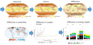
This dataset represents the impact of climate change on renewable energy supply potentials and is based on the study by Gernaat et al., 2021. The data has been used in a NAVIGATE activity focussed at representing climate change impacts in an integrated assessment model (IMAGE) (Van Vuuren et al., in preparation).

Data description

The approach by Gernaat et al. (2021) is schematically shown in Figure 1. They first created climate- and spatially explicit energy supply estimates that are subsequently translated to regional cost-supply curves. The dataset contains the extended data underlying the figures in Gernaat et al., (2021), including geographically-explicit changes in energy supply potentials by energy carrier, as well as cost-supply curves (see list below).

The data is based on the output from 2  General Circulation Models (GCMs), HadGEM2-ES and IPSL-CM5A-LR, for the following climatic parameters: solar irradiance (kWh m^-2 day^-1), temperature (°C), sugar cane and maise yields (t ha^-1 y^-1), wind speed (m s^-1), and runoff (kg m^-2 s^-1). The lignocellulosic crop yields (t ha^-1 y^-1) were computed here following the ISIMIP2b protocol. For this, the model mean was calculated for the historical period and 2070–2100. The climate data were used as input to calculate renewable energy potential. This includes the theoretical potential, which is the upper limit of the resource availability based on biophysical conditions. In subsequent steps, this theoretical potential is constrained by geographical and technical restrictions. Geographical restrictions reduce the theoretical potential of available and suitable areas for energy production. For bioenergy, this means the exclusion of nature reserves, forests, water-scarce areas, and areas used for agriculture. Similar restrictions are also applied to other renewable technologies. To the remaining geographical area, further technical restrictions have been applied. The climate impacts were calculated for historical and future periods using the ISIMIP2b database. The maps of technical potential, combined with economic information, have been used to generate cost-supply curves. These curves show the cumulative technical potential against the production cost, showing that the cost of production in each location depends on its productivity. Cost-supply curves are widely used in IAMs to model the long-term cost development of renewable energy technologies. These curves indicate resource depletion, as the most productive sites are slowly being depleted, and thus higher cost-incurring sites need to be used.

Figure 1: Schematic overview of the approach in Gernaat et al., 2021. 

Description of the datafiles (description from Gernaat et al., 2021):

Source Data Fig. 1

Model mean (GFLD-ESM2M, HadGEM2-ES, IPSL-CM5A-LR and MIROC5) historical (1970–2000), RCP2.6 (2070–2100) and RCP6.0 (2070–2100) climate input data: Solar irradiance (kWh m−2 per day) (global horizontal), temperature (°C), wind speed (m s−1), runoff (kg m−2 s−1), sugar cane and maize yields (t ha−1 yr−1) and lignocellulosic crop yields (switchgrass and Miscanthus, or trees) (t ha−1 yr−1).

Source Data Fig. 2

Technical potential per GCM for the historical (1970–2000) period, and the future RCP2.6 (2070–2100) and RCP6.0 (2070–2100) periods: utility-scale PV and rooftop PV, concentrated solar power (CSP), pnshore and offshore wind energy, hydropower, first-generation bioenergy, and lignocellulosic bioenergy with and without CO2 fertilization.

Source Data Fig. 3

Technical potential per region, GCM and RCP for: utility-scale PV and rooftop PV, concentrated solar power (CSP), onshore and offshore wind energy, hydropower, first-generation bioenergy, and lignocellulosic bioenergy with and without CO2 fertilization.

Source Data Fig. 4

Primary energy supply (2071–2100) based on historical, RCP2.6 and RCP6.0 climate with and without CO2 fertilization (PJ).

Source Data Extended Data Fig. 1

Model mean (GFLD-ESM2M, HadGEM2-ES, IPSL-CM5A-LR and MIROC5) historical (1970–2000), RCP2.6 (2070–2100) and RCP6.0 (2070–2100) climate input data: solar irradiance (kWh m−2 per day) (global horizontal), temperature (°C), wind speed (m s−1), runoff (kg m−2 s−1), sugar cane and maize yields (t ha−1 yr−1) and lignocellulosic crop yields (switchgrass and Miscanthus, or trees) (t ha−1 yr−1).

Source Data Extended Data Fig. 2

Model mean (GFLD-ESM2M, HadGEM2-ES, IPSL-CM5A-LR and MIROC5) historical (1970–2000), RCP2.6 (2070–2100) and RCP6.0 (2070–2100) climate input data: solar irradiance (kWh m−2 per day) (global horizontal), temperature (°C), wind speed (m s−1), runoff (kg m−2 s−1), sugar cane and maize yields (t ha−1 yr−1) and lignocellulosic crop yields (switchgrass and Miscanthus, or trees) (t ha−1 yr−1).

Source Data Extended Data Fig. 4

Technical potential per GCM for the historical (1970–2000) period, and the future RCP2.6 (2070–2100) and RCP6.0 (2070–2100) periods: utility-scale PV and rooftop PV, concentrated solar power (CSP), pnshore and offshore wind energy, hydropower, first-generation bioenergy, and lignocellulosic bioenergy with and without CO2 fertilization.

Source Data Extended Data Fig. 5

Technical potential per region, GCM and RCP for: utility-scale PV and rooftop PV, concentrated solar power (CSP), onshore and offshore wind energy, hydropower, first-generation bioenergy, and lignocellulosic bioenergy with and without CO2 fertilization.

Source Data Extended Data Fig. 7

Primary energy supply (2071–2100) based on historical, RCP2.6 and RCP6.0 climate with and without CO2 fertilization (PJ).

Source Data Extended Data Fig. 8

Primary energy supply (2071–2100) based on historical, RCP2.6 and RCP6.0 climate with and without CO2 fertilization (PJ).

Source Data Extended Data Fig. 9

Primary energy supply (2071–2100) based on historical, RCP2.6 and RCP6.0 climate with and without CO2 fertilization (PJ).

Source Data Extended Data Fig. 10

Primary energy supply (2071–2100) based on historical, RCP2.6 and RCP6.0 climate with and without CO2 fertilization (PJ).

Link to data

Climate change impacts on renewable energy supply | Nature Climate Change

How to use the data

The dataset contains NetCDF and and CSV files, which can be used separately for analysis purposes and/or implemented in integrated assessment models.

License information

The study has been published open access under a Creative Commons license. The data can be freely used by all parties.

Publications

Gernaat, D. E. H. J., de Boer, H. S., Daioglou, V., Yalew, S. G., Müller, C., & van Vuuren, D. P. (2021). Climate change impacts on renewable energy supply [Article]. Nature Climate Change, 11(2), 119-125. https://doi.org/10.1038/s41558-020-00949-9

Van Vuuren et al., 2024 (in preparation), A more complete image: Enhancing the climate change impact representation in integrated assessment models. Detlef P. van Vuuren, Mathijs Harmsen, Isabela Tagomori, Astrid Bos, Jonathan Doelman, Lotte de Vos, Kaj-Ivar van der Wijst, Geanderson Ambrósio, Harmen-Sytze de Boer, Vassilis Daioglou, David Gernaat, Elke Stehfest

This dataset represents the impact of climate change on labour productivity using five Exposure Response Functions (ERFs) based on changes in Wet Bulb Globe Temperature (WBGT). The data has been used in a NAVIGATE activity focussed at representing climate change impacts in an integrated assessment model (IMAGE) (Van Vuuren et al., in preparation).

Data description

Climate change has an impact on labour productivity as workers experiencing severe heat stress tend to slow down and take more breaks for rehydration and cooling, resulting in reduced performance during working hours. We refer to this as a reduction in labour productivity. This dataset presents the results of an assessment on the impact of climate change on labour productivity using five different Exposure Response Functions (ERFs). The ERFs were established based on changes in Wet Bulb Globe Temperature (WBGT) and cover a range of work intensities that occur in different working environments. The functional forms and scope of the ERFs are different, with some showing continuous decreases in productivity with increasing WBGT and others showing decreases in discrete steps. Most of the models demonstrate saturation with increasing WBGT at different levels. The dataset emphasizes the need to consider saturation effects when aggregating the results of individual models. The dataset is a result of the study titled “Effects of climate change on combined labour productivity and supply: an empirical, multi-model study”(Dasgupta et al. 2021).

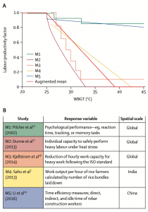
Figure 1: Exposure-response functions for labour productivity (A) The five individual exposure response functions from selected impact models used to calculate the augmented mean response function (red line) used to quantify the effect of WBGT (°C) on labour productivity in this study. (B) Labour productivity impact models, with their response variable and spatial scale.

Link to data

N.a.

How to use the data

This dataset provides annual estimates of reductions in labour productivity from 2006-2100, relative to the baseline period of 1986-2005, at both country and grid level. Specifically, the dataset includes relative reductions in labour productivity for four different climate models (HadGEM2-ES, GFDL-ESM2M, MIROC5, and IPSL-CM5A-LR) under two different scenarios (RCP2.6 and RCP6.0), as well as absolute reductions in labour productivity for IPSL-CM5A-LR under the same scenarios. The dataset also provides results for high, medium, and low exposure sectors. This information can be useful for assessing the potential impacts of climate change on labour productivity in various sectors and regions.

License information

The study has been published open access under a Creative Commons license. The data can be freely used by all parties.

Publications

Dasgupta, Shouro et al. 2021. “Effects of Climate Change on Combined Labour Productivity and Supply: An Empirical, Multi-Model Study.” The Lancet Planetary Health 5(7): e455–65.

Van Vuuren et al., 2024 (in preparation), A more complete image: Enhancing the climate change impact representation in integrated assessment models. Detlef P. van Vuuren, Mathijs Harmsen, Isabela Tagomori, Astrid Bos, Jonathan Doelman, Lotte de Vos, Kaj-Ivar van der Wijst, Geanderson Ambrósio, Harmen-Sytze de Boer, Vassilis Daioglou, David Gernaat, Elke Stehfest

This dataset represents the impact of climate change on heating and cooling demand (or heating and cooling degree days, HDD CDD). The data has been used in a NAVIGATE activity focussed at representing climate change impacts in an integrated assessment model (IMAGE) (Van Vuuren et al., in preparation).

Data description

The dataset contains regional cooling and heating demand days, based on the study by Byers et al. (2018) who derived their climate data from an ensemble of downscaled and bias-corrected global climate models (ISIMIP2). The data has been prepared for the climate impact study in the NAVIGATE project (by Edward Byers, IIASA, 11 Feb 2021 – byers@iiasa.ac.at). The data is provided for RCP2.6 and RCP6.0, i.e., emission pathways reaching 2.6W/m² and 6.0W/m² forcing levels in 2100. The data represents gridded global surface air temperature data at the daily resolution, summarized to decadal timesteps and a monthly mean and subsequently aggregated to ISO countries, population weighted by SSP population. The data is based on the results of 4 global circulation models (GCMs): GFDL, HadGEM, IPSL, MIROC5. The population data is based on Jones & O’Neill (2016).

Link to data

Data to download here.

How to use the data

The (.csv) data is suitable to be implemented in integrated assessment models. In the NAVIGATE climate impact exercise, it was used in the the IMAGE energy model (TIMER), which could be a useful approach for similar models. Based on the data, “CDD/HDD as a function of global mean temperature” coefficients were derived that ran internally in TIMER and which scaled with the level of projected warming.

License information

The study has been published open access under a Creative Commons license. The data can be freely used by all parties.

Publications

Byers, E., Gidden, M., Leclere, D., Balkovic, J., Burek, P., Ebi, K., Greve, P., Grey, D., Havlik, P., Hillers, A., Johnson, N., Kahil, T., Krey, V., Langan, S., Nakicenovic, N., Novak, R., Obersteiner, M., Pachauri, S., Palazzo, A., . . . Riahi, K. (2018). Global exposure and vulnerability to multi-sector development and climate change hotspots [Article]. Environmental Research Letters, 13(5), Article 055012. https://doi.org/10.1088/1748-9326/aabf45

Lange, S.: Trend-preserving bias adjustment and statistical downscaling with ISIMIP3BASD (v1.0), Geosci. Model Dev., 12, 3055–3070, https://doi.org/10.5194/gmd-12-3055-2019, 2019.

B Jones and B C O’Neill 2016 Environ. Res. Lett. 11 084003 DOI 10.1088/1748-9326/11/8/084003

Van Vuuren et al., 2024 (in preparation), A more complete image: Enhancing the climate change impact representation in integrated assessment models. Detlef P. van Vuuren, Mathijs Harmsen, Isabela Tagomori, Astrid Bos, Jonathan Doelman, Lotte de Vos, Kaj-Ivar van der Wijst, Geanderson Ambrósio, Harmen-Sytze de Boer, Vassilis Daioglou, David Gernaat, Elke Stehfest

LIFE is an empirically-based model of low-carbon lifestyles that characterises populations into four lifestyle groups of varying sizes. Each group varies in the strength of its low-carbon values and norms, and its propensity towards low-carbon behaviours.

LIFE is designed to allow IAMs to endogenously simulate lifestyle change. LIFE provides information on lifestyle heterogeneity and behavioural propensities towards low-carbon lifestyle change; these modify IAM equations that generate behavioural outcomes, which in turn feed back to LIFE to modify the sizes and behavioural propensities of the different lifestyle groups.

This work was demonstrated in NAVIGATE in an implementation with MESSAGEiX-Buildings, written up as an open access journal article in Environmental Research Letters. The underlying conceptualisation of low-carbon lifestyles is published as a journal article in WIREs Energy and Environment. The empirical analysis behind the LIFE model is published as a journal article in Global Environmental Change.

In addition, the empirical analysis of national social statistics that underpins the LIFE model is also available here. We have also made available a here summarising the full work flow.

Link to code

License information

This tool / short code, written in Python, contains 1) calculations of 6 key diagnostic indicators of the behaviour of integrated assessment models (IAMs) based on IAM output (as described in Harmsen et al., 2021) and 2) code to create graphs that visualize the diagnostic results for multiple IAMs. The tool is a useful asset for IAM modellers that want to perform diagnostic analyses with their model or with multiple models. As described in Harmsen et al.:

“Integrated assessment models (IAMs) form a prime tool in informing about climate mitigation strategies. Diagnostic indicators that allow comparison across these models can help describe and explain differences in model projections. This increases transparency and comparability. Earlier, the IAM community has developed an approach to diagnose models (Kriegler et al., 2015). Here we build on this, by proposing a selected set of well-defined indicators as a community standard, to systematically and routinely assess IAM behaviour, similar to metrics used for other modeling communities such as climate models. These indicators are the relative abatement index, emission reduction type index, inertia timescale, fossil fuel reduction, transformation index and cost per abatement value. We apply the approach to 17 IAMs, assessing both older as well as their latest versions, as applied in the IPCC 6th Assessment Report. The study shows that the approach can be easily applied and used to indentify key differences between models and model versions. Moreover, we demonstrate that this comparison helps to link model behavior to model characteristics and assumptions. We show that together, the set of six indicators can provide useful indication of the main traits of the model and can roughly indicate the general model behavior.”

Code description

The code contains calculations of the 6 key indicators and scripts to create graphs based on the indicator output.

The tool also includes the dataset used in the Harmsen et al. paper.

Link to code/data

Link to the code and data (By: Kaj-Ivar van der Wijst, 2021)

https://doi.org/10.5281/zenodo.5727623

How to use the tool

The tool also includes the dataset used in the Harmsen et al. paper and can thus be run directly without external input. However, if the code is used to add diagnostic results for new models or new model versions, it is necessary to run the diagnostic scenarios with these models first and to add the scenario results to the dataset in the tool. The diagnostic scenarios have a very simple setup. Models are confronted with a stylized carbon price profile. The diagnostic indicators are based on the model outcomes in 2050. See the Harmsen et al. paper for a description of the scenarios and indicators, or contact Mathijs.harmsen@pbl.nl.

License information

The underlying study has been published open access under a Creative Commons licence. The data can be freely used by all parties.

Publications

Harmsen, M. et al (2021) Integrated assessment model diagnostics: key indicators and model evolution. Environ. Res. Lett. 16 054046. https://doi.org/10.1088/1748-9326/abf964

Link to the code and data (By: Kaj-Ivar van der Wijst, 2021), https://doi.org/10.5281/zenodo.5727623